Basic synthetic control tutorial

Video overview

AI summary

The lecture discusses synthetic controls, a method of causal inference for analyzing policy changes when only one unit is treated. A data-driven counterfactual is constructed using an algorithm. Inference is challenging due to the lack of a conventional control group.

00:00 Synthetic controls is a method of causal inference for policy changes

05:39 Synthetic control method matches pre-trends to estimate treatment effect

10:38 Synthetic control studies assume treated units remain treated and spillovers are excluded.

15:38 Weights in synthetic controls are determined by an algorithm

20:40 Synthetic controls is a standard minimization procedure used for causal inference.

25:12 Synthetic control method matches characteristics of Basque country well

29:47 Synthetic control studies require careful consideration of methodological refinements.

01:21 Conventional standard errors don’t work for synthetic controls

Detailed Summary for Causal Inference – 22/23 – Synthetic Control I by Merlin

00:00 Synthetic controls is a method of causal inference for policy changes

Synthetic controls is used when only one unit has been treated
The method constructs a data-driven counterfactual using an algorithm

05:39 Synthetic control method matches pre-trends to estimate treatment effect

Weighted average of control units chosen by algorithm
Assumption of parallel trends in absence of treatment

10:38 Synthetic control studies assume treated units remain treated and spillovers are excluded.

Counterfactuals are weighted averages of actual outcomes of units in the donor pool.
Treatment effects are estimated by comparing actual outcomes of treated units to synthetic controls.

15:38 Weights in synthetic controls are determined by an algorithm

Characteristics of treated unit and control units are matched based on multiple variables
Vector of weights is found to minimize distance between target variables

20:40 Synthetic controls is a standard minimization procedure used for causal inference.

Weighted variables are counted as separate variables.
Simple minimization algorithm typically matches pre-trends well.

25:12 Synthetic control method matches characteristics of Basque country well

Synthetic control algorithm finds weights based on variables like GDP and education
Weight only rests on two regions: Catalonia and Madrid

29:47 Synthetic control studies require careful consideration of methodological refinements.

Matching on pre-treatment outcomes is crucial for finding a good match.
Statistical inference in synthetic control studies is challenging and requires careful consideration.

01:21 Conventional standard errors don’t work for synthetic controls

Synthetic controls have high serial correlation and only two clusters
Non-parametric methods like placebo synthetic controls are needed for meaningful standard errors

AI summary

The lecture discusses the difficulty in drawing inference in synthetic control studies and suggests using non-parametric methods based on permutation tests. An example of the tobacco control program in California is used to illustrate this.

00:00 Non-parametric methods based on permutation tests are used for inference in synthetic control studies.

05:50 Synthetic California is a meaningful counterfactual

11:16 Graphs show the difference between treated and synthetic control unit.

16:18 California is a clear outlier in placebo estimates

01:26 When running a synthetic control study, it’s important to add one to each numerator and denominator to avoid false statistical significance.

01:06 Brexit vote caused UK GDP to fall below its doppelganger

31:08 Synthetic control method is a powerful tool for policy evaluation

36:10 Synthetic control meets machine learning through matrix completion methods.

Detailed Summary for Causal Inference – 23/23 – Synthetic Control II by Merlin

00:00 Non-parametric methods based on permutation tests are used for inference in synthetic control studies.

Synthetic control studies compare the time series of the outcome of the treated unit to that of the synthetic control unit.
Matching is done based on a restricted donor pool and a few pre-periods and cross-sectional variables.

05:50 Synthetic California is a meaningful counterfactual

Synthetic California has a small difference compared to actual California
Matching on a pre-period considerably before treatment kicks in provides a plausible research design

11:16 Graphs show the difference between treated and synthetic control unit.

38 states were used to estimate synthetic controls and treatment effects.
Observations with huge pre-treatment differences were trimmed.

16:18 California is a clear outlier in placebo estimates

Empirical p-value is computed by counting how many placebo estimates are greater than California’s
Consideration of values in opposite direction makes it equivalent to a two-sided test

01:26 When running a synthetic control study, it’s important to add one to each numerator and denominator to avoid false statistical significance.

Adding one to each numerator and denominator gives a more accurate p-value.
Many papers get this wrong, so it’s important to be aware of this issue.

01:06 Brexit vote caused UK GDP to fall below its doppelganger - Using placebo, timing of Brexit vote was analyzed - Robustness checks and expectation augmented VAR model were used for analysis

31:08 Synthetic control method is a powerful tool for policy evaluation

Synthetic control method compares treated unit with a weighted average of control units
Results are robust to different donor pool restrictions and can complement other methods

36:10 Synthetic control meets machine learning through matrix completion methods.

Abadi and Jeremy Luer devised a method to choose between multiple optimal synthetic controls using machine learning.
Methodological refinements include dealing with imperfect pre-treatment matches and covariate imbalance, with augmented estimators providing bounds on estimates.

Video source: Ben Elsner

This note is based on the article “Synth: An R Package for Synthetic Control Methods in Comparative Case Studies” by Alberto Abadie, Alexis Diamond, and Jens Hainmueller, which introduces the Synth package in R. This package implements synthetic control methods used in comparative case studies. These methods construct a synthetic control unit as weighted average of available control units that best approximate the relevant characteristics of the treated unit prior to the treatment. The Synth package includes functions such as synth(), which constructs the synthetic control unit, and dataprep(), which organizes the data. Other functions like synth.tables(), path.plot(), and gaps.plot() help in summarizing and illustrating the results. The authors demonstrate the use of these functions with an example from a study on the economic effects of conflict in the Basque Country using other Spanish regions as potential control units. They conclude by discussing future extensions to the Synth package

Introduction

Introduction to Social Science Research Methods

Social science often explores causal questions about the impacts of historical events and policy interventions on aggregate units like cities, regions, and countries.
Comparative case studies are a common method for answering these questions, comparing outcomes for affected units (treated group) with unaffected units (control group).

Limitations of Traditional Comparative Case Studies

Traditional methods leave control unit selection to the analyst, raising questions about selection arbitrariness and the credibility of control units as proxies for treated units’ counterfactual outcomes.

Introduction to Synthetic Control Methods

Synthetic control methods, introduced by Abadie and Gardeazabal (2003) and Abadie et al. (2010), address these issues by proposing a data-driven control-group selection procedure, a framework for assessing the chosen control group’s suitability, and a means of producing quantitative inference.
A synthetic control unit is defined as a weighted average of available control units that approximates the treated unit’s relevant characteristics prior to treatment.
The synthetic control method guards against extrapolation outside the convex hull of the data, as weights from all control units can be chosen to be positive and sum to one.

The Synth Package in R

The Synth package in R implements synthetic control methods, with the central function being synth(), which constructs the synthetic control unit by solving an optimization problem to identify a set of weights assigned to potential control units.
Other functions like dataprep(), synth.tables(), path.plot(), and gaps.plot() help organize data, summarize results, and create visual representations.

Case Study: The Basque Country

The data example from Abadie and Gardeazabal (2003) uses synthetic control methods to investigate the effects of the terrorist conflict in the Basque Country on the Basque economy, using other Spanish regions as potential control units.

Synthetic control methods

Synthetic Control Methods Overview

Synthetic control methods involve creating synthetic control units from multiple control units. The weights defining the synthetic control unit are chosen to best approximate the characteristics of the treated unit during the pre-treatment period.
The synthetic control method is used to estimate the outcomes that would have been observed for the treated unit in the absence of the intervention.

Theoretical Properties

The method is based on an econometric model that generalizes the usual difference-in-differences model commonly applied in empirical literature.

Construction of Synthetic Control Units

The synthetic control unit is constructed from a set of control units, known as the donor pool. The intervention occurs at a specific time period, dividing the timeline into pre-intervention and post-intervention periods.
Two potential outcomes are defined: the outcome if the unit is not exposed to the intervention (denoted as \(Y_{i t}^{N}\)), and the outcome if the unit is exposed to the intervention (denoted as \(Y_{i t}^{I}\)). The goal is to estimate the effect of the intervention on the outcome for the treated unit in the post-intervention period, formally defined as the difference between the two potential outcomes \(\alpha_{1 t}=Y_{1 t}^{I}-Y_{1 t}^{N}\) for periods \(T_{0}+1, T_{0}+2, \ldots, T\).

Estimation of Missing Potential Outcome

The synthetic control method aims to construct a synthetic control group that provides a reasonable estimate for the missing potential outcome \(Y_{i t}^{N}\) for the treated unit in the post-intervention period.

Weight Selection

The synthetic control unit is defined by a vector of weights, each representing a particular weighted average of control units. The weights are chosen to best approximate the unit exposed to the intervention with respect to the outcome predictors and linear combinations of pre-intervention outcomes.
In empirical applications, the weights are chosen so that the identity conditions hold approximately. The user can easily check how similar a particular synthetic control unit is to the treated unit.

Numerical Implementation

The synth() function is used to numerically implement the synthetic control estimator. It defines a distance between the synthetic control unit and the treated unit, and chooses the vector of weights to minimize this distance.
The synth() function allows for flexibility in the choice of the matrix V, which allows different weights to the variables depending on their predictive power on the outcome. An optimal choice of V minimizes the mean square error of the synthetic control estimator.

Inferential Techniques

Synthetic control methods facilitate inferential techniques akin to permutation tests that are well-suited to comparative case studies in which the number of units in the comparison group and the number of periods in the sample are relatively small.
The method proposes conducting placebo studies by iteratively applying the synthetic control method by randomly reassigning the intervention in time or across units to produce a set of placebo effects. These effects are then compared to the effect estimated for the actual intervention.
The placebo tests are akin to permutation inference, where a test statistic is iteratively computed under random permutations of the assignment vector that determines whether a unit is in the treatment or the control group.

Implementation of the `Synth` package

Abadie and Gardeazabal (2003) study the economic impacts of conflict in the Basque Country.
A synthetic Basque Country was constructed using a combination of other Spanish regions, which closely resembled the Basque Country’s economic characteristics before the onset of political terrorism in the 1970s.
The data, spanning from 1955 to 1997, covers 17 Spanish regions, excluding the small autonomous towns of Ceuta and Melilla on the African coast.
The data includes per-capita GDP (the outcome variable), as well as population density, sectoral production, investment, and human capital (the predictor variables).
Missing data in the dataset are denoted by NA.

library(Synth)
library(SCtools)
library(tidyverse)
library(skimr)

 data("basque")

 basque[85:89, 1:4]

   regionno regionname year   gdpcap
85        2  Andalucia 1996 5.995930
86        2  Andalucia 1997 6.300986
87        3     Aragon 1955 2.288775
88        3     Aragon 1956 2.445159
89        3     Aragon 1957 2.603399

head(basque)

  regionno     regionname year   gdpcap sec.agriculture sec.energy sec.industry
1        1 Spain (Espana) 1955 2.354542              NA         NA           NA
2        1 Spain (Espana) 1956 2.480149              NA         NA           NA
3        1 Spain (Espana) 1957 2.603613              NA         NA           NA
4        1 Spain (Espana) 1958 2.637104              NA         NA           NA
5        1 Spain (Espana) 1959 2.669880              NA         NA           NA
6        1 Spain (Espana) 1960 2.869966              NA         NA           NA
  sec.construction sec.services.venta sec.services.nonventa school.illit
1               NA                 NA                    NA           NA
2               NA                 NA                    NA           NA
3               NA                 NA                    NA           NA
4               NA                 NA                    NA           NA
5               NA                 NA                    NA           NA
6               NA                 NA                    NA           NA
  school.prim school.med school.high school.post.high popdens invest
1          NA         NA          NA               NA      NA     NA
2          NA         NA          NA               NA      NA     NA
3          NA         NA          NA               NA      NA     NA
4          NA         NA          NA               NA      NA     NA
5          NA         NA          NA               NA      NA     NA
6          NA         NA          NA               NA      NA     NA

glimpse(basque)

Rows: 774
Columns: 17
$ regionno              <dbl> 1, 1, 1, 1, 1, 1, 1, 1, 1, 1, 1, 1, 1, 1, 1, 1, …
$ regionname            <chr> "Spain (Espana)", "Spain (Espana)", "Spain (Espa…
$ year                  <dbl> 1955, 1956, 1957, 1958, 1959, 1960, 1961, 1962, …
$ gdpcap                <dbl> 2.354542, 2.480149, 2.603613, 2.637104, 2.669880…
$ sec.agriculture       <dbl> NA, NA, NA, NA, NA, NA, 19.54, NA, 19.05, NA, 16…
$ sec.energy            <dbl> NA, NA, NA, NA, NA, NA, 4.71, NA, 4.31, NA, 4.31…
$ sec.industry          <dbl> NA, NA, NA, NA, NA, NA, 26.42, NA, 26.05, NA, 27…
$ sec.construction      <dbl> NA, NA, NA, NA, NA, NA, 6.27, NA, 6.83, NA, 7.64…
$ sec.services.venta    <dbl> NA, NA, NA, NA, NA, NA, 36.62, NA, 38.00, NA, 38…
$ sec.services.nonventa <dbl> NA, NA, NA, NA, NA, NA, 6.44, NA, 5.77, NA, 6.48…
$ school.illit          <dbl> NA, NA, NA, NA, NA, NA, NA, NA, NA, 2863.278, 28…
$ school.prim           <dbl> NA, NA, NA, NA, NA, NA, NA, NA, NA, 18679.10, 18…
$ school.med            <dbl> NA, NA, NA, NA, NA, NA, NA, NA, NA, 1064.246, 11…
$ school.high           <dbl> NA, NA, NA, NA, NA, NA, NA, NA, NA, 359.7457, 37…
$ school.post.high      <dbl> NA, NA, NA, NA, NA, NA, NA, NA, NA, 212.1434, 21…
$ popdens               <dbl> NA, NA, NA, NA, NA, NA, NA, NA, NA, NA, NA, NA, …
$ invest                <dbl> NA, NA, NA, NA, NA, NA, NA, NA, NA, 18.36018, 20…

skim(basque)

Data summary
Name	basque
Number of rows	774
Number of columns	17
_______________________
Column type frequency:
character	1
numeric	16
________________________
Group variables	None

Variable type: character

skim_variable	n_missing	complete_rate	min	max	empty	n_unique	whitespace
regionname	0	1	6	28	0	18	0

Variable type: numeric

skim_variable	n_missing	complete_rate	mean	sd	p0	p25	p50	p75	p100	hist
regionno	0	1.00	9.50	5.19	1.00	5.00	9.50	14.00	18.00	▇▆▇▆▇
year	0	1.00	1976.00	12.42	1955.00	1965.00	1976.00	1987.00	1997.00	▇▇▇▇▇
gdpcap	0	1.00	5.39	2.24	1.24	3.69	5.34	6.87	12.35	▅▇▇▂▁
sec.agriculture	684	0.12	20.27	10.38	1.32	13.54	19.24	27.48	46.50	▅▇▇▅▂
sec.energy	684	0.12	5.19	4.04	1.60	2.70	3.67	6.08	21.36	▇▂▁▁▁
sec.industry	684	0.12	23.92	9.28	9.56	17.81	23.14	27.48	46.22	▅▇▆▂▂
sec.construction	684	0.12	7.21	1.36	4.34	6.24	7.13	8.18	11.28	▃▇▆▅▁
sec.services.venta	684	0.12	36.49	7.26	26.23	31.25	34.75	39.19	58.21	▇▇▃▁▂
sec.services.nonventa	684	0.12	6.93	1.98	3.43	5.50	6.68	7.93	13.11	▃▇▃▂▁
school.illit	666	0.14	308.05	630.84	8.10	40.29	116.23	252.27	2863.28	▇▁▁▁▁
school.prim	666	0.14	2118.52	4216.78	151.32	432.29	852.13	1763.31	19459.56	▇▁▁▁▁
school.med	666	0.14	145.61	297.45	8.61	26.51	47.75	119.04	1696.15	▇▁▁▁▁
school.high	666	0.14	45.94	92.11	3.06	9.13	16.70	38.76	474.94	▇▁▁▁▁
school.post.high	666	0.14	25.46	51.58	1.66	4.41	7.71	19.06	252.25	▇▁▁▁▁
popdens	756	0.02	105.77	101.52	22.38	44.77	80.38	122.57	442.45	▇▂▁▁▁
invest	198	0.74	21.40	4.11	9.33	18.74	21.35	23.75	39.41	▁▇▇▁▁

In Abadie and Gardeazabal (2003), there are 16 control regions and the 13 predictor variables:

1964-1969 averages for gross total investment/GDP (invest).
1964-1969 averages for the share of education:
- 1964-1969 averages for the share of the working-age population that was illiterate (school.illit)
- 1964-1969 averages for the share of the working-age population with up to primary school education (school.prim)
- 1964-1969 averages for the share of the working-age population with some high school (school.med)
- 1964-1969 averages for the share of the working-age population wit high school (school.high)
1961-1969 averages for six industrial-sector shares as a percentage of total production (these variables are named with a sec. prefix). These variables are available on a biennial basis \((1961,1963, \ldots, 1969)\)
1960-1969 averages for real GDP per-capita (gdpcap) measured in thousands of 1986 USD.
1969 population density measured in persons per square kilometer (popdens).

Using `dataprep()`

At a minimum, synth() requires as inputs the four data matrices: \(X_{1}, X_{0}, Z_{1}\), and \(Z_{0}\). In our example, these four data matrices are:

\(X_{1}\) is the \((13 \times 1)\) vector of Basque region predictors
\(X_{0}\) is the \((13 \times 16)\) matrix of values of the same variables for the 16 control regions. Note that all but one of these predictors is an average value over some range of the pre-treatment period, and the precise date-range varies across predictor variables.
\(Z_{1}\) is a \((10 \times 1)\) vector which contain the values for the outcome variable for the Basque country
\(Z_{0}\) is a \((10 \times 16)\) matrix which contain the values for the outcome variable for the control units for the 10 pre-intervention periods over which we want to minimize the MSPE.

It is strongly recommended to use dataprep() to extract and package the inputs for synth() in a single list object. This list object is also used by other functions such as synth.tables(), path.plot(), and gaps.plot() to produce tables and figures that illustrate the results

To obtain \(X_{1}\) and \(X_{0}\) the user must define the predictor variables, the operator (e.g., mean), and time-period (e.g., 1964:1969) applied to these variables.
The user must specify the dependent variable (e.g., gdpcap), the variable(s) identifying unit names (e.g., regionname) and/or numbers (e.g., regionno), the variable identifying time-periods (e.g., year), the treated unit (e.g., region number 17 which is the Basque country), the control units (e.g., regions number \(c(2: 16,18))\), the time-period over which to optimize (e.g., the pre-treatment period 1960:1969). This refers to \(Z_{1}\) and \(Z_{0}\) accordingly.
The user should also specify time-period over which outcome data should be plotted (usually before and after treatment, e.g., \(1955:1997\) )

How to use the function dataprep()

Some of the predictor information is given by the arguments predictors, predictors.op, and time.predictors.prior.
The rest of the information for the other predictors is specified in the special.predictors list.

This separation allow for easy handling of several predictors with the same operator over the same pre-treatment period (in this case, the school and investment variables) as well as additional custom (or “special”) predictors with heterogeneous operators and time-periods. For example, the variables for the sector production shares (with the sec prefix) are only available on a biennial basis \((1961,1963, \ldots, 1969)\) extracted via seq \((1961,1969,2)\). Averaging over the available years is easily accommodated using the special.predictors list. For more details and examples check the help file of dataprep().

# Prepare the data for analysis
dataprep.out <- dataprep(
  foo = basque,  # the dataset to be prepared
  
  # the predictor variables to be used in the model
  predictors = c("school.illit", "school.prim", "school.med", 
                 "school.high", "school.post.high", "invest"),
  
  predictors.op = "mean",  # operation to be applied on the predictors
  
  time.predictors.prior = 1964:1969,  # time period for the predictors
  
  # special predictors with their respective time periods and operations
  special.predictors = list(
    list("gdpcap", 1960:1969, "mean"),
    list("sec.agriculture", seq(1961,1969,2), "mean"),
    list("sec.energy", seq(1961,1969,2), "mean"),
    list("sec.industry", seq(1961,1969,2), "mean"),
    list("sec.construction", seq(1961,1969,2), "mean"),
    list("sec.services.venta", seq(1961,1969,2), "mean"),
    list("sec.services.nonventa", seq(1961,1969,2), "mean"),
    list("popdens", 1969, "mean")
  ),
  
  dependent = "gdpcap",  # the dependent variable
  
  unit.variable = "regionno",  # the variable representing the unit of observation
  
  unit.names.variable = "regionname",  # the variable representing the names of the units
  
  time.variable = "year",  # the variable representing the time period
  
  treatment.identifier = 17,  # the identifier for the treatment group
  
  controls.identifier = c(2:16,18),  # the identifiers for the control groups
  
  time.optimize.ssr = 1960:1969,  # the time period over which the sum of squared residuals (SSR) is minimized to estimate the weights
  
  time.plot = 1955:1997  # the time period for the plot
)

We can confirm the contents of the four data matrices:

\(X_1\) contains the predictors of the treatment unit (region 17).
Education-related predictors are averaged over the 1964-1969 period.
GPDpc averaged over the 1960-1969 period is also included as a predictor.
Sector-related predictors are averaged over the 1961-1969 period (on a biannual basis).
Population density is only available for the year 1969.

dataprep.out$X1

                                                 17
school.illit                              39.888465
school.prim                             1031.742299
school.med                                90.358668
school.high                               25.727525
school.post.high                          13.479720
invest                                    24.647383
special.gdpcap.1960.1969                   5.285468
special.sec.agriculture.1961.1969          6.844000
special.sec.energy.1961.1969               4.106000
special.sec.industry.1961.1969            45.082000
special.sec.construction.1961.1969         6.150000
special.sec.services.venta.1961.1969      33.754000
special.sec.services.nonventa.1961.1969    4.072000
special.popdens.1969                     246.889999

Notice that dataprep.out appends the associated date-range only to the names of the special.predictors.

In \(X_0\): - Region 1 is not included because it is national value - Region 17 is not included because it is the treatment unit.

dataprep.out$X0

                                                  2          3          4
school.illit                             863.389160  73.121226  31.488423
school.prim                             3062.424886 728.578929 670.909393
school.med                               155.565318  44.215389  46.398482
school.high                               57.266496  16.091676  14.799358
school.post.high                          27.278924   8.684416   6.424505
invest                                    19.320031  21.577486  22.769643
special.gdpcap.1960.1969                   2.560747   3.699907   3.733876
special.sec.agriculture.1961.1969         24.194000  21.726000  12.362000
special.sec.energy.1961.1969               2.774000   6.278000  18.648000
special.sec.industry.1961.1969            18.276000  22.780000  24.126000
special.sec.construction.1961.1969         8.130000   7.832000   9.006000
special.sec.services.venta.1961.1969      38.186000  34.289999  30.152000
special.sec.services.nonventa.1961.1969    8.444000   7.096000   5.708000
special.popdens.1969                      68.510002  24.040001  98.739998
                                                 5          6          7
school.illit                             47.903906 128.308287   9.394911
school.prim                             300.813619 522.094955 289.571732
school.med                               20.045204  45.447489  24.106414
school.high                               5.921604  12.086849   7.304420
school.post.high                          3.680154   5.844122   2.885214
invest                                   24.441712  25.954247  29.071211
special.gdpcap.1960.1969                  5.215974   3.051014   3.871173
special.sec.agriculture.1961.1969        13.130000  19.944000  15.922000
special.sec.energy.1961.1969              2.076000   7.818000   2.894000
special.sec.industry.1961.1969           18.258000   9.816000  36.530000
special.sec.construction.1961.1969        8.294000   8.670000   5.976000
special.sec.services.venta.1961.1969     51.752000  45.278001  33.484000
special.sec.services.nonventa.1961.1969   6.494000   8.482000   5.198000
special.popdens.1969                    104.169998 148.250000  87.389999
                                                  8           9          10
school.illit                             105.508144  254.449707  277.935237
school.prim                             1766.928691 1035.269368 2883.361735
school.med                               102.299929   33.369543  215.165476
school.high                               37.787317   16.539727   63.608315
school.post.high                          19.173427    6.308165   32.374611
invest                                    19.652509   17.970690   22.520380
special.gdpcap.1960.1969                   2.807062    2.240688    5.147008
special.sec.agriculture.1961.1969         29.718000   36.086001    6.936000
special.sec.energy.1961.1969               7.818000    5.180000    2.880000
special.sec.industry.1961.1969            16.474000   17.178000   40.056000
special.sec.construction.1961.1969         7.144000    5.810000    6.706000
special.sec.services.venta.1961.1969      30.844000   29.238000   39.068000
special.sec.services.nonventa.1961.1969    8.000000    6.506000    4.356000
special.popdens.1969                      28.770000   22.379999  153.119995
                                                 11         12          13
school.illit                             266.967601 177.727966  234.752001
school.prim                             1695.117126 692.888550 1666.930420
school.med                               103.959094  24.048450   77.464478
school.high                               34.275772  11.271676   29.341941
school.post.high                          16.822106   4.570566   13.543060
invest                                    23.702696  20.239484   20.606269
special.gdpcap.1960.1969                   3.843245   1.926478    2.516288
special.sec.agriculture.1961.1969         18.582000  37.948000   28.862000
special.sec.energy.1961.1969               2.698000   2.646000    5.328000
special.sec.industry.1961.1969            28.046000  10.886000   17.882000
special.sec.construction.1961.1969         6.170000   8.770000    7.032000
special.sec.services.venta.1961.1969      39.064001  31.720000   33.714001
special.sec.services.nonventa.1961.1969    5.444000   8.038000    7.188000
special.popdens.1969                     128.699997  28.969999   91.019997
                                                 14         15         16
school.illit                             133.158962 105.877481  13.438050
school.prim                             1856.074280 431.746806 280.002396
school.med                               269.961647  27.907434  20.450936
school.high                               62.458658   9.082540   6.550353
school.post.high                          57.704985   4.428528   4.190368
invest                                    16.234543  20.706271  19.955159
special.gdpcap.1960.1969                   5.976692   2.899557   3.996087
special.sec.agriculture.1961.1969          1.864000  19.352000  24.704000
special.sec.energy.1961.1969               2.074000  10.228000   2.740000
special.sec.industry.1961.1969            23.834000  19.644000  28.398000
special.sec.construction.1961.1969         8.358000   6.290000   6.982000
special.sec.services.venta.1961.1969      52.714000  36.177999  30.468000
special.sec.services.nonventa.1961.1969   11.162000   8.312000   6.710000
special.popdens.1969                     442.450012  73.360001  44.169998
                                                18
school.illit                              9.151832
school.prim                             152.269465
school.med                                9.760035
school.high                               3.377170
school.post.high                          1.732763
invest                                   18.055932
special.gdpcap.1960.1969                  3.809205
special.sec.agriculture.1961.1969        30.322001
special.sec.energy.1961.1969              2.888000
special.sec.industry.1961.1969           26.612000
special.sec.construction.1961.1969        5.238000
special.sec.services.venta.1961.1969     28.300000
special.sec.services.nonventa.1961.1969   6.644000
special.popdens.1969                     46.580002

\(Z_1\) contains the outcome values of the treatment unit BEFORE treatment (that is 1960-1969).

 dataprep.out$Z1

           17
1960 4.285918
1961 4.574336
1962 4.898957
1963 5.197015
1964 5.338903
1965 5.465153
1966 5.545916
1967 5.614896
1968 5.852185
1969 6.081405

\(Z_0\) contains the outcome values of the control units BEFORE treatment (that is 1960-1969).

 dataprep.out$Z0

            2        3        4        5        6        7        8        9
1960 2.010140 2.881462 2.967295 4.058841 2.357684 3.137032 2.138817 1.667524
1961 2.129177 3.099543 3.143887 4.360254 2.445730 3.327621 2.239503 1.752428
1962 2.280348 3.359183 3.373536 4.646173 2.648243 3.555341 2.454227 1.920451
1963 2.431020 3.614182 3.597258 4.911525 2.844759 3.771423 2.672237 2.091902
1964 2.508855 3.680091 3.672594 5.050700 2.951157 3.839403 2.777778 2.182591
1965 2.584690 3.745287 3.743359 5.184662 3.054199 3.906098 2.882176 2.274707
1966 2.694444 3.883319 3.909383 5.466795 3.231791 4.032133 2.988075 2.378392
1967 2.802342 4.016138 4.073122 5.737646 3.403385 4.155955 3.094544 2.482362
1968 2.987361 4.243645 4.308626 6.161454 3.660312 4.375893 3.302271 2.709083
1969 3.179092 4.476221 4.549700 6.581691 3.912882 4.610826 3.520994 2.947444
           10       11       12       13       14       15       16       18
1960 4.241788 3.219294 1.535847 1.983290 5.161097 2.118609 3.163525 2.969866
1961 4.575335 3.362468 1.596258 2.005784 5.632605 2.305484 3.335904 3.153171
1962 4.838046 3.569980 1.705584 2.185661 5.840831 2.521422 3.623393 3.404384
1963 5.081334 3.765210 1.817695 2.366395 6.024493 2.739074 3.894816 3.669238
1964 5.158098 3.823693 1.882819 2.458797 6.099329 2.851257 3.985147 3.803985
1965 5.223651 3.874179 1.948872 2.549700 6.152028 2.965938 4.072979 3.921808
1966 5.332477 3.978149 2.032633 2.669666 6.110469 3.099186 4.210011 4.032705
1967 5.429449 4.073408 2.117609 2.787846 6.057341 3.227292 4.352399 4.160311
1968 5.674379 4.279777 2.245501 2.978363 6.253142 3.461154 4.556984 4.373036
1969 5.915524 4.486290 2.381962 3.177378 6.435590 3.706155 4.765710 4.603542

There may be instances where it’s beneficial to adjust and alter \(X_{0}\) and \(X_{1}\) directly, without referring back to the original dataset. For instance, consider the five distinct education variables (school.illit, school.prim, school.med, school.high, school.post.high), which denote the count of individuals with different education levels, in thousands. In their 2003 study, Abadie and Gardeazabal combined the two highest categories (school.high and school.post.high) to represent all individuals with education beyond high school. They also used the percentage share for each predictor instead of the total count of individuals. The subsequent code demonstrates how to merge these variables in both \(X_{0}\) and \(X_{1}\), and how to convert the relevant values into percentage distributions:

# Combine 'school.high' and 'school.post.high' in X1 and X0 matrices
dataprep.out$X1["school.high",] <- dataprep.out$X1["school.high",] + dataprep.out$X1["school.post.high",]
dataprep.out$X0["school.high",] <- dataprep.out$X0["school.high",] + dataprep.out$X0["school.post.high",]

# Remove 'school.post.high' from X1 and X0 matrices
post_high_row <- which(rownames(dataprep.out$X1)=="school.post.high")
dataprep.out$X1 <- as.matrix(dataprep.out$X1[-post_high_row,])
dataprep.out$X0 <- as.matrix(dataprep.out$X0[-post_high_row,])

# Find the indices of 'school.illit' and 'school.high' in X0 matrix
illit_row_index <- which(rownames(dataprep.out$X0)=="school.illit")
high_row_index  <- which(rownames(dataprep.out$X0)=="school.high")

# Scale the values in the rows between 'school.illit' and 'school.high' in X1 and X0 matrices to percentages
dataprep.out$X1[illit_row_index:high_row_index,] <- (100*dataprep.out$X1[illit_row_index:high_row_index,]) / sum(dataprep.out$X1[illit_row_index:high_row_index,])
dataprep.out$X0[illit_row_index:high_row_index,] <- 100*scale(dataprep.out$X0[illit_row_index:high_row_index,], center=FALSE, scale=colSums(dataprep.out$X0[illit_row_index:high_row_index,]))

Running `synth()`

The function synth() identifies the synthetic control for the Basque region by determining the weight vector \(W^{*}\), which is achieved by solving the nested optimization problem outlined in equations (1) and (2).

\[ \left\|X_{1}-X_{0} W\right\|_{V}=\sqrt{\left(X_{1}-X_{0} W\right)^{\prime} V\left(X_{1}-X_{0} W\right)} \hspace{1cm} (1) \]

\[ \arg \min _{V \in \mathcal{V}}\left(Z_{1}-Z_{0} W^{*}(V)\right)^{\prime}\left(Z_{1}-Z_{0} W^{*}(V)\right) \hspace{1cm} (2) \]

For any given \(V\), the function synth() locates a \(W^{*}(V)\) by minimizing equation (1). This minimization is achieved using a constrained quadratic optimization function from the kernlab package in R. The function synth() then determines the diagonal matrix \(V^{*}\) that minimizes equation (2), thereby minimizing the Mean Squared Prediction Error (MSPE) for the pre-intervention period. To solve the optimization problem presented in equation (2), the authors utilize the general-purpose optimization function optim() in R.

 synth.out <- synth(data.prep.obj = dataprep.out,
                    method = "BFGS" #   set optim() to use the BFGS quasi-Newton algorithm. 
                    )


X1, X0, Z1, Z0 all come directly from dataprep object.


**************** 
 searching for synthetic control unit  
 

**************** 
**************** 
**************** 

MSPE (LOSS V): 0.008864629 

solution.v:
 0.01556809 0.001791073 0.04417159 0.03409436 8.45063e-05 0.2009836 0.09484592 0.007689227 0.1339499 0.008723866 0.009680737 0.1081257 0.3402913 

solution.w:
 4.92e-08 5.17e-08 1.352e-07 2.85e-08 5.32e-08 5.177e-07 5.24e-08 7.29e-08 0.8507986 2.274e-07 4.03e-08 9.51e-08 0.1491998 5.61e-08 9.02e-08 1.061e-07

Obtaining Results: Tables, Figures, and Estimates

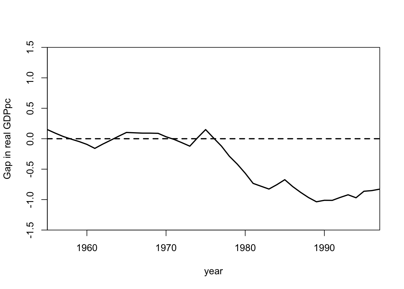
The annual discrepancies in the GPD trend between the Basque region and its synthetic control

 gaps <- dataprep.out$Y1plot - (dataprep.out$Y0plot %*% synth.out$solution.w)
 gaps[1:3, 1]

      1955       1956       1957 
0.15021896 0.09166384 0.03714761

gaps

               17
1955  0.150218957
1956  0.091663836
1957  0.037147612
1958 -0.006003578
1959 -0.045912501
1960 -0.093028265
1961 -0.158741268
1962 -0.088701802
1963 -0.025035609
1964  0.040376216
1965  0.102991299
1966  0.097365414
1967  0.091767963
1968  0.091457295
1969  0.088290338
1970  0.032164161
1971 -0.010718484
1972 -0.065240285
1973 -0.122248917
1974  0.018114662
1975  0.149837948
1976  0.012249750
1977 -0.121311425
1978 -0.287951073
1979 -0.417501286
1980 -0.566472165
1981 -0.733650764
1982 -0.780284226
1983 -0.826525640
1984 -0.754859524
1985 -0.672982676
1986 -0.785770335
1987 -0.880817969
1988 -0.966277731
1989 -1.035845236
1990 -1.011476539
1991 -1.012419501
1992 -0.964326371
1993 -0.920837104
1994 -0.969747353
1995 -0.863014218
1996 -0.851919587
1997 -0.828080864

Tables are produced by using the synth.tab() function:

 synth.tables <- synth.tab(dataprep.res = dataprep.out,
                           synth.res    = synth.out
                           )

This function produces four different types of tables:

 names(synth.tables)

[1] "tab.pred" "tab.v"    "tab.w"    "tab.loss"

tab.pred compares pre-treatment predictor values for the treated unit, the synthetic control unit, and all the units in the sample.

synth.tables$tab.pred

                                        Treated Synthetic Sample Mean
school.illit                              3.321     7.645      10.983
school.prim                              85.893    82.285      80.911
school.med                                7.522     6.965       5.427
school.high                               3.264     3.105       2.679
invest                                   24.647    21.583      21.424
special.gdpcap.1960.1969                  5.285     5.271       3.581
special.sec.agriculture.1961.1969         6.844     6.179      21.353
special.sec.energy.1961.1969              4.106     2.760       5.310
special.sec.industry.1961.1969           45.082    37.636      22.425
special.sec.construction.1961.1969        6.150     6.952       7.276
special.sec.services.venta.1961.1969     33.754    41.104      36.528
special.sec.services.nonventa.1961.1969   4.072     5.371       7.111
special.popdens.1969                    246.890   196.288      99.414

The synthetic Basque country is fairly similar to the real Basque country. The sample means of the predictor variables over the 16 control regions are provided as a comparison.

tab.v shows the weight corresponding to each predictor

 synth.tables$tab.v

                                        v.weights
school.illit                            0.016    
school.prim                             0.002    
school.med                              0.044    
school.high                             0.034    
invest                                  0        
special.gdpcap.1960.1969                0.201    
special.sec.agriculture.1961.1969       0.095    
special.sec.energy.1961.1969            0.008    
special.sec.industry.1961.1969          0.134    
special.sec.construction.1961.1969      0.009    
special.sec.services.venta.1961.1969    0.01     
special.sec.services.nonventa.1961.1969 0.108    
special.popdens.1969                    0.34

tab.v shows the weight corresponding to each potential control unit

 synth.tables$tab.w

   w.weights                   unit.names unit.numbers
2      0.000                    Andalucia            2
3      0.000                       Aragon            3
4      0.000       Principado De Asturias            4
5      0.000             Baleares (Islas)            5
6      0.000                     Canarias            6
7      0.000                    Cantabria            7
8      0.000              Castilla Y Leon            8
9      0.000           Castilla-La Mancha            9
10     0.851                     Cataluna           10
11     0.000         Comunidad Valenciana           11
12     0.000                  Extremadura           12
13     0.000                      Galicia           13
14     0.149        Madrid (Comunidad De)           14
15     0.000           Murcia (Region de)           15
16     0.000 Navarra (Comunidad Foral De)           16
18     0.000                   Rioja (La)           18

We see that Cataluna contributes 85 percent and Madrid contributes 15 percent to the synthetic Basque country; a zero weight is assigned to all the other control regions.

 path.plot(synth.res = synth.out,
           dataprep.res = dataprep.out,
           Ylab = "Real GDPpc",
           Xlab = "year",
           Ylim = c(0,12),
           Legend = c("Basque country","synthetic Basque country"),
           Legend.position = "bottomright"
           )

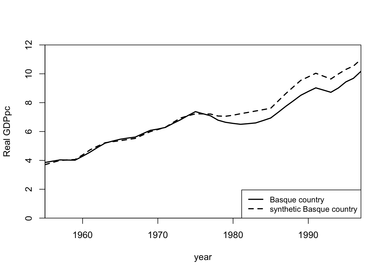
We know that for the Basque country, terrorism claimed its first victim in 1968, but large scale terrorist activity only began in the mid-70s.

The gaps.plot() function shows how the difference between treated and synthetic control outcomes change over time.

 gaps.plot(synth.res = synth.out,
           dataprep.res = dataprep.out,
           Ylab = "Gap in real GDPpc",
           Xlab = "year",
           Ylim = c(-1.5,1.5),
           Main = NA
           )

Placebo tests

dataprep.out <-
              dataprep(foo = basque,
                       predictors = c("school.illit" , "school.prim" , "school.med" ,
                                      "school.high" , "school.post.high" , "invest") ,
                       predictors.op = "mean" ,
                       time.predictors.prior = 1964:1969 ,
                       special.predictors = list(
                         list("gdpcap" , 1960:1969 , "mean"),
                         list("sec.agriculture" ,      seq(1961,1969,2), "mean"),
                         list("sec.energy" ,           seq(1961,1969,2), "mean"),
                         list("sec.industry" ,         seq(1961,1969,2), "mean"),
                         list("sec.construction" ,     seq(1961,1969,2), "mean"),
                         list("sec.services.venta" ,   seq(1961,1969,2), "mean"),
                         list("sec.services.nonventa" ,seq(1961,1969,2), "mean"),
                         list("popdens", 1969, "mean")
                                                ),
                       dependent = "gdpcap",
                       unit.variable = "regionno",
                       unit.names.variable = "regionname",
                       time.variable = "year",
                       treatment.identifier = 10, # Change the ID to other unit that did NOT receive the treatment
                       controls.identifier = c(2:9,11:16,18),
                       time.optimize.ssr = 1960:1969,
                       time.plot = 1955:1997
                       )

# Combine 'school.high' and 'school.post.high' in X1
dataprep.out$X1["school.high",] <- dataprep.out$X1["school.high",] + dataprep.out$X1["school.post.high",]

# Remove 'school.post.high' from X1
dataprep.out$X1 <- as.matrix(dataprep.out$X1[-which(rownames(dataprep.out$X1)=="school.post.high"),])

# Combine 'school.high' and 'school.post.high' in X0
dataprep.out$X0["school.high",] <- dataprep.out$X0["school.high",] + dataprep.out$X0["school.post.high",]

# Remove 'school.post.high' from X0
dataprep.out$X0 <- dataprep.out$X0[-which(rownames(dataprep.out$X0)=="school.post.high"),]

# Find the row indices for 'school.illit' and 'school.high'
lowest  <- which(rownames(dataprep.out$X0)=="school.illit")
highest <- which(rownames(dataprep.out$X0)=="school.high")

# Convert the values in X1 from 'school.illit' to 'school.high' into percentage shares
dataprep.out$X1[lowest:highest,] <- (100*dataprep.out$X1[lowest:highest,]) / sum(dataprep.out$X1[lowest:highest,])

# Scale the values in X0 from 'school.illit' to 'school.high' and convert into percentages
dataprep.out$X0[lowest:highest,] <- 100*scale(dataprep.out$X0[lowest:highest,], center=FALSE, scale=colSums(dataprep.out$X0[lowest:highest,]))

synth.out <- synth(data.prep.obj = dataprep.out,
                   method = "BFGS"
                   )


X1, X0, Z1, Z0 all come directly from dataprep object.


**************** 
 searching for synthetic control unit  
 

**************** 
**************** 
**************** 

MSPE (LOSS V): 0.0003093975 

solution.v:
 0.01405753 0.01342444 0.00503692 0.001792628 0.07939864 0.5166646 0.2816736 0.08745663 1.02215e-05 1.72355e-05 2.00017e-05 0.000439494 7.9985e-06 

solution.w: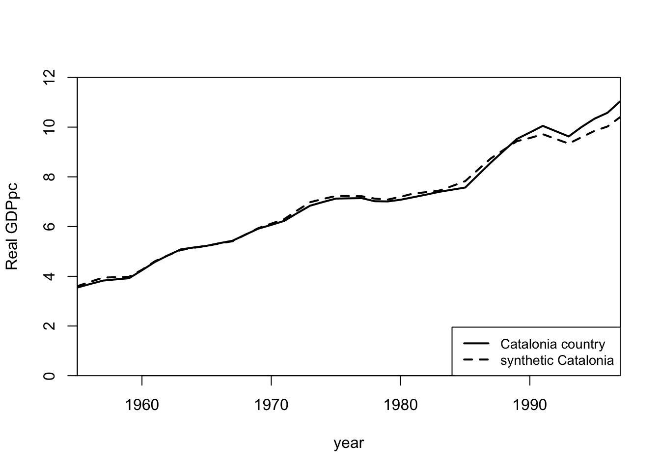
 1.09249e-05 7.4848e-06 0.03590867 0.271566 1.48966e-05 0.2574606 3.0579e-06 2.6666e-06 2.53122e-05 2.2184e-06 4.9234e-06 0.4349691 1.81685e-05 3.5539e-06 2.4453e-06

path.plot(synth.res = synth.out,
          dataprep.res = dataprep.out,
          tr.intake = NA,
          Ylab = "Real GDPpc",
          Xlab = "year",
          Ylim = c(0,12),
          Legend = c("Catalonia country","synthetic Catalonia"),
          Legend.position = "bottomright",
          )

 gaps.plot(synth.res = synth.out,
           dataprep.res = dataprep.out,
           Ylab = "Gap in real GDPpc",
           Xlab = "year",
           Ylim = c(-1.5,1.5),
           Main = NA
           )

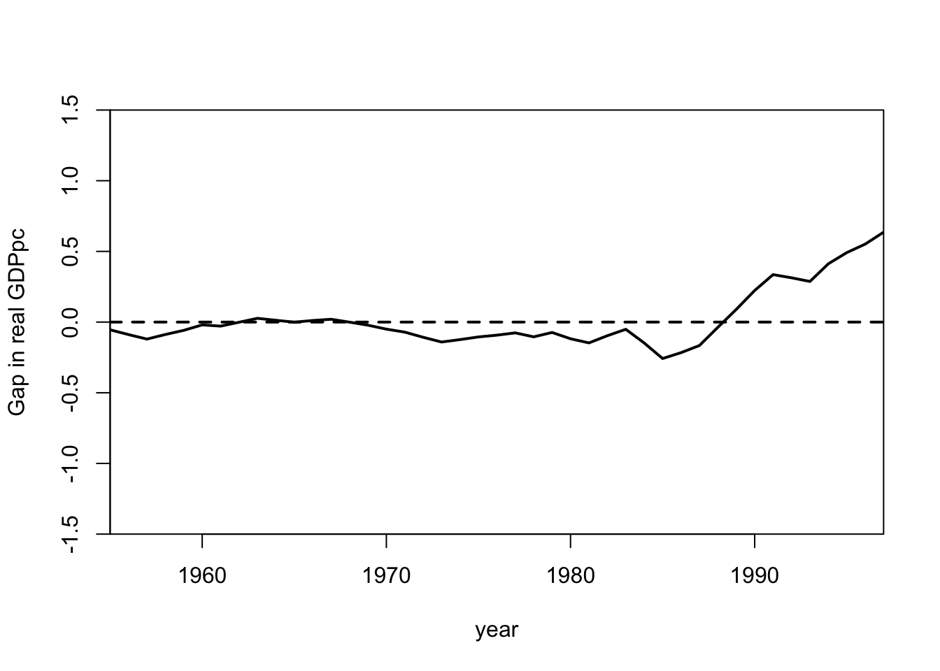
Synthetic control methods are beneficial because they allow for placebo tests. These tests reassign the intervention to units and periods where it didn’t occur to test the method’s effectiveness.
Abadie and Gardeazabal (2003) demonstrated the placebo test for the synthetic control method using Catalonia as an example. They showed that there was no identifiable treatment effect when the synthetic control method was applied to Catalonia.
There are several types of placebo tests that can be run with this package, such as placebos-in-time and placebos with outcome variables that should be unaffected by the treatment.
Users can perform exact inferential techniques similar to permutation tests by applying the synthetic control method to every control unit in the sample and collecting information on the gaps.
The user can plot these gaps to visually determine whether the line associated with the true synthetic control unit conspicuously differentiates itself from the rest.
The approach is implemented by running a for loop to implement placebo tests across all control units in the sample and collecting information on the gaps.
The results of this inferential technique can be seen in the figure below, where regions with a poor fit for the pre-treatment period are excluded.
The figure demonstrates that when exposure to terrorism is reassigned to other regions, there is a very low probability of obtaining a gap as large as the one obtained for the Basque region.
Poor-fitting regions are usually those that are very unusual in their pre-treatment characteristics, so no combination of other regions in the sample can reproduce the pre-treatment trends for these regions.
An alternative to excluding regions based on MPSE is to compute the distribution of the ratio of post- to pre-treatment MPSE.

store <- matrix(NA,length(1955:1997),17)
colnames(store) <- unique(basque$regionname)[-1]

# run placebo test
for(iter in 2:18)
 {
 dataprep.out <-
              dataprep(foo = basque,
                       predictors = c("school.illit" , "school.prim" , "school.med" ,
                                      "school.high" , "school.post.high" , "invest") ,
                       predictors.op = "mean" ,
                       time.predictors.prior = 1964:1969 ,
                       special.predictors = list(
                         list("gdpcap" , 1960:1969 , "mean"),
                         list("sec.agriculture" ,      seq(1961,1969,2), "mean"),
                         list("sec.energy" ,           seq(1961,1969,2), "mean"),
                         list("sec.industry" ,         seq(1961,1969,2), "mean"),
                         list("sec.construction" ,     seq(1961,1969,2), "mean"),
                         list("sec.services.venta" ,   seq(1961,1969,2), "mean"),
                         list("sec.services.nonventa" ,seq(1961,1969,2), "mean"),
                         list("popdens", 1969, "mean")
                                                ),
                       dependent = "gdpcap",
                       unit.variable = "regionno",
                       unit.names.variable = "regionname",
                       time.variable = "year",
                       treatment.identifier = iter,
                       controls.identifier = c(2:18)[-iter+1],
                       time.optimize.ssr = 1960:1969,
                       time.plot = 1955:1997
                       )




 dataprep.out$X1["school.high",] <-
   dataprep.out$X1["school.high",] + dataprep.out$X1["school.post.high",]
 dataprep.out$X1 <-
   as.matrix(dataprep.out$X1[-which(rownames(dataprep.out$X1)=="school.post.high"),])
 dataprep.out$X0["school.high",] <-
   dataprep.out$X0["school.high",] + dataprep.out$X0["school.post.high",]
 dataprep.out$X0 <-
   dataprep.out$X0[-which(rownames(dataprep.out$X0)=="school.post.high"),]

 lowest  <- which(rownames(dataprep.out$X0)=="school.illit")
 highest <- which(rownames(dataprep.out$X0)=="school.high")

 dataprep.out$X1[lowest:highest,] <-
  (100*dataprep.out$X1[lowest:highest,]) /
   sum(dataprep.out$X1[lowest:highest,])
 dataprep.out$X0[lowest:highest,] <-
   100*scale(dataprep.out$X0[lowest:highest,],
             center=FALSE,
             scale=colSums(dataprep.out$X0[lowest:highest,])
  )

# run synth
synth.out <- synth(
                   data.prep.obj = dataprep.out,
                   method = "BFGS"
                   )

# store gaps
store[,iter-1] <- dataprep.out$Y1plot - (dataprep.out$Y0plot %*% synth.out$solution.w)
}


X1, X0, Z1, Z0 all come directly from dataprep object.


**************** 
 searching for synthetic control unit  
 

**************** 
**************** 
**************** 

MSPE (LOSS V): 9.769789e-06 

solution.v:
 0.1623716 0.08905496 0.09211519 0.1037775 0.04294261 0.09945295 0.02249312 0.1194742 0.03049302 0.1169147 0.07851873 0.001934032 0.04045739 

solution.w:
 4.669e-07 3.74e-08 0.06871975 0.09930165 1.441e-07 2.547e-07 0.08792619 2.2712e-06 2.52271e-05 0.6027934 1.2071e-06 0.04270843 0.09852008 3.265e-07 7.13e-08 4.937e-07 


X1, X0, Z1, Z0 all come directly from dataprep object.


**************** 
 searching for synthetic control unit  
 

**************** 
**************** 
**************** 

MSPE (LOSS V): 0.0007759196 

solution.v:
 0.07626995 0.06396751 0.04486642 0.005179403 0.1468072 0.1395639 0.04849465 0.02590254 0.3192316 0.1271959 0.001595317 8.09127e-05 0.0008446376 

solution.w:
 0.002847392 0.1942325 0.1397633 0.000914255 0.02097697 0.1304587 0.004124095 0.08064028 0.00442945 0.1654631 1.32207e-05 0.00022504 0.002175287 0.2469207 0.003732397 0.00308341 


X1, X0, Z1, Z0 all come directly from dataprep object.


**************** 
 searching for synthetic control unit  
 

**************** 
**************** 
**************** 

MSPE (LOSS V): 0.0005444699 

solution.v:
 0.01231921 9.531e-07 0.1099582 0.08532242 0.04666882 0.0801413 0.1406802 0.06732613 0.1100789 0.1234673 0.007544381 0.09789709 0.1185951 

solution.w:
 1.53e-08 0.4234967 4.8e-09 0.3944335 9e-09 9.14e-08 2.78e-08 5.01e-08 2.25e-08 1.03e-08 3.59e-08 2.8e-09 3.1662e-06 0 0.1820663 1e-08 


X1, X0, Z1, Z0 all come directly from dataprep object.


**************** 
 searching for synthetic control unit  
 

**************** 
**************** 
**************** 

MSPE (LOSS V): 0.1186101 

solution.v:
 3.33288e-05 0.02256084 7.02905e-05 0.00728127 0.01570196 0.5482453 0.000157174 0.1427547 1.75687e-05 0.008580386 0.0194893 0.2209856 0.01412218 

solution.w:
 0.0004961839 2.6461e-06 2.1e-09 0.08641808 0.0002997258 9.362e-07 2.4951e-06 0.6565079 0.0009040657 5.63022e-05 3.1999e-06 0.2552986 4.115e-07 6.7063e-06 1e-10 2.769e-06 


X1, X0, Z1, Z0 all come directly from dataprep object.


**************** 
 searching for synthetic control unit  
 

**************** 
**************** 
**************** 

MSPE (LOSS V): 0.001323248 

solution.v:
 0.07393106 0.1211972 0.0001074404 0.0002131637 0.05120843 0.4328742 0.03867743 0.09524453 0.05366269 0.02123013 3.23276e-05 0.1113294 0.0002920094 

solution.w:
 1.22945e-05 9.7347e-06 2.8878e-05 0.1714208 6.9274e-06 7.4741e-06 1.2302e-06 1.1608e-06 3.3878e-06 0.2501338 7.9401e-06 2.5312e-06 0.5783608 1.8927e-06 2.639e-07 8.676e-07 


X1, X0, Z1, Z0 all come directly from dataprep object.


**************** 
 searching for synthetic control unit  
 

**************** 
**************** 
**************** 

MSPE (LOSS V): 0.0001164363 

solution.v:
 0.0003310047 0.00213788 0.05690954 0.001834906 0.1001146 0.3631324 0.0704808 0.130847 0.0003822926 0.006252639 0.05395768 0.0008783568 0.212741 

solution.w:
 3.71e-08 0.08179105 4.7e-09 0.0007733517 0.2397046 1.116e-07 5.7e-08 2.653e-07 0.5196322 6.15e-08 4.81e-08 5.2e-09 6.3e-08 1.5131e-06 0.1580965 1.92e-07 


X1, X0, Z1, Z0 all come directly from dataprep object.


**************** 
 searching for synthetic control unit  
 

**************** 
**************** 
**************** 

MSPE (LOSS V): 0.0007839866 

solution.v:
 0.02451637 0.1180743 3.00186e-05 0.002431598 0.05720764 0.2808197 0.08189894 1.56597e-05 0.2487468 0.04979899 0.01211177 0.07946989 0.04487829 

solution.w:
 8.4712e-06 0.004654015 0.05866539 2.86957e-05 2.36318e-05 2.2085e-06 1.6e-09 2.3678e-06 3.039e-06 0.001702417 0.7675253 6.07913e-05 6.5852e-06 0.0004907144 1.5026e-06 0.1668249 


X1, X0, Z1, Z0 all come directly from dataprep object.


**************** 
 searching for synthetic control unit  
 

**************** 
**************** 
**************** 

MSPE (LOSS V): 0.003441637 

solution.v:
 0.2819977 3.77076e-05 0.007304756 0.1913337 0.001234845 0.1077445 0.0001339538 0.2506414 0.01139748 0.01475026 0.0008777025 0.0002952483 0.1322507 

solution.w:
 7.3e-09 7.62e-08 4e-09 4.4e-08 3e-10 2.636e-07 1.562e-07 1.301e-07 1.3078e-06 0.6608552 0.0127187 5e-10 0.3263682 8.03e-08 3.22e-08 5.57476e-05 


X1, X0, Z1, Z0 all come directly from dataprep object.


**************** 
 searching for synthetic control unit  
 

**************** 
**************** 
**************** 

MSPE (LOSS V): 0.001731602 

solution.v:
 0.04854086 0.01447919 0.0005696063 4.6529e-06 0.4545145 0.1743639 0.1425628 0.006164227 0.109689 0.01319099 0.03525773 0.0003438238 0.000318642 

solution.w:
 0.09820231 2.5384e-06 1.3516e-06 0.0001096605 1.17957e-05 1.188e-06 9.979e-07 2.457e-07 6.69951e-05 1.6059e-06 1.6941e-06 0.1862123 1.95324e-05 9.556e-07 0.7153662 5.738e-07 


X1, X0, Z1, Z0 all come directly from dataprep object.


**************** 
 searching for synthetic control unit  
 

**************** 
**************** 
**************** 

MSPE (LOSS V): 0.005472465 

solution.v:
 0.1142611 0.1418908 0.00463412 0.02252889 0.1341089 0.1908037 0.02291209 0.009698626 0.0640444 0.04711843 0.02584312 0.1773129 0.04484299 

solution.w:
 6.6007e-06 5.4245e-06 2.299e-06 0.004242197 0.1641151 0.1883559 3.3363e-06 0.2476481 0.3954618 4.6418e-06 1.09237e-05 3.2388e-06 2.77576e-05 5.0792e-06 9.71674e-05 1.0437e-05 


X1, X0, Z1, Z0 all come directly from dataprep object.


**************** 
 searching for synthetic control unit  
 

**************** 
**************** 
**************** 

MSPE (LOSS V): 0.1146395 

solution.v:
 0.02427409 0.01026832 0.1489549 0.1368267 0.001135408 0.1606203 0.4393701 0.03087507 0.01231399 8.552e-07 0.0001460941 0.003204566 0.03200954 

solution.w:
 9.72e-08 4.31e-08 1.28e-08 1.83e-08 9.18e-08 4.29e-08 2.558e-07 0.9999989 1.22e-08 3.36e-08 1.428e-07 1.5e-09 3.53e-08 9.67e-08 1.17e-08 1.699e-07 


X1, X0, Z1, Z0 all come directly from dataprep object.


**************** 
 searching for synthetic control unit  
 

**************** 
**************** 
**************** 

MSPE (LOSS V): 0.0004619251 

solution.v:
 0.01229623 0.05637697 0.1650633 0.2219118 0.0001000538 0.4147641 0.0001505474 0.06202615 5.54293e-05 0.01398409 3.1358e-06 0.05287225 0.0003960339 

solution.w:
 1.44024e-05 0.0001065384 0.009454045 0.0003189615 6.8995e-06 0.07434963 0.3488591 0.3598222 0.000879104 0.0002847956 0.2045495 2.347e-07 6.8642e-06 3.45546e-05 0.0001249696 0.00118827 


X1, X0, Z1, Z0 all come directly from dataprep object.


**************** 
 searching for synthetic control unit  
 

**************** 
**************** 
**************** 

MSPE (LOSS V): 0.5308454 

solution.v:
 0.05175466 0.01526417 0.1909266 0.04978537 0.1337012 0.04370974 0.2253978 0.04765019 0.0003084564 0.04816708 0.04571619 0.00414232 0.1434762 

solution.w:
 1.19e-08 3.6e-09 5.1e-09 1.65e-08 1.36e-08 1e-10 3.7e-09 6e-10 5.54e-08 1.9e-09 1e-10 2e-09 6e-09 2.04e-08 0.9999999 7.7e-09 


X1, X0, Z1, Z0 all come directly from dataprep object.


**************** 
 searching for synthetic control unit  
 

**************** 
**************** 
**************** 

MSPE (LOSS V): 0.001910045 

solution.v:
 0.08721003 0.1577794 0.07246097 0.08734601 0.001628194 0.07553655 0.09820718 0.1465568 0.001400442 0.03045952 0.05526499 0.135878 0.05027189 

solution.w:
 8.69e-08 1.163e-07 0.1163706 2.44e-08 0.600644 1.58e-08 2.181e-07 0.2829842 2.87e-08 5.59e-08 7.2e-09 7.85e-08 3.964e-07 2.84e-08 1.56e-08 7.08e-08 


X1, X0, Z1, Z0 all come directly from dataprep object.


**************** 
 searching for synthetic control unit  
 

**************** 
**************** 
**************** 

MSPE (LOSS V): 0.0002241912 

solution.v:
 0.07026391 0.08293033 0.04596517 0.0001588333 0.05633258 0.05478577 2.3875e-05 0.08468431 0.2554776 0.112146 0.1737682 0.01777752 0.04568584 

solution.w:
 1.56678e-05 0.4373507 7.32e-08 8.2582e-06 4.0295e-06 9.5503e-06 0.000224769 3.3315e-06 1.43698e-05 5.4561e-06 9.89416e-05 1.07651e-05 0.00200689 2.4195e-06 0.1560405 0.4042042 


X1, X0, Z1, Z0 all come directly from dataprep object.


**************** 
 searching for synthetic control unit  
 

**************** 
**************** 
**************** 

MSPE (LOSS V): 0.008864629 

solution.v:
 0.01556809 0.001791073 0.04417159 0.03409436 8.45063e-05 0.2009836 0.09484592 0.007689227 0.1339499 0.008723866 0.009680737 0.1081257 0.3402913 

solution.w:
 4.92e-08 5.17e-08 1.352e-07 2.85e-08 5.32e-08 5.177e-07 5.24e-08 7.29e-08 0.8507986 2.274e-07 4.03e-08 9.51e-08 0.1491998 5.61e-08 9.02e-08 1.061e-07 


X1, X0, Z1, Z0 all come directly from dataprep object.


**************** 
 searching for synthetic control unit  
 

**************** 
**************** 
**************** 

MSPE (LOSS V): 0.0006965933 

solution.v:
 0.1115345 0.1004851 0.01632611 0.02227407 0.01271669 0.1144789 0.001231086 0.1444595 0.1168052 1.07937e-05 0.1738477 0.04247705 0.1433533 

solution.w:
 8.388e-06 1.02366e-05 0.0001290961 2.4275e-06 3.6204e-06 1.6069e-06 0.04234802 0.07727088 1.01873e-05 1.10019e-05 8.1453e-06 5.66883e-05 2.7544e-06 1.03189e-05 0.8800848 4.18468e-05

# now do figure
data <- store
rownames(data) <- 1955:1997

# Set bounds in gaps data
gap.start     <- 1
gap.end       <- nrow(data)
years         <- 1955:1997
gap.end.pre  <- which(rownames(data)=="1969")

#  MSPE Pre-Treatment
mse        <-             apply(data[ gap.start:gap.end.pre,]^2,2,mean)
basque.mse <- as.numeric(mse[16])
# Exclude states with 5 times higher MSPE than basque
data <- data[,mse<5*basque.mse]
Cex.set <- .75

# Plot
plot(years,data[gap.start:gap.end,which(colnames(data)=="Basque Country (Pais Vasco)")],
     ylim=c(-2,2),xlab="year",
     xlim=c(1955,1997),ylab="Gap in real GDPpc",
     type="l",lwd=2,col="black",
     xaxs="i",yaxs="i")

# Add lines for control states
for (i in 1:ncol(data)) { lines(years,data[gap.start:gap.end,i],col="gray") }

## Add Basque Line
lines(years,data[gap.start:gap.end,which(colnames(data)=="Basque Country (Pais Vasco)")],lwd=2,col="black")

# Add grid
abline(v=1970,lty="dotted",lwd=2)
abline(h=0,lty="dashed",lwd=2)
legend("bottomright",legend=c("Basque country","control regions"),
lty=c(1,1),col=c("black","gray"),lwd=c(2,1),cex=.8)
arrows(1967,-1.5,1968.5,-1.5,col="black",length=.1)
text(1961.5,-1.5,"Terrorism Onset",cex=Cex.set)
abline(v=1955)
abline(v=1997)
abline(h=-2)
abline(h=2)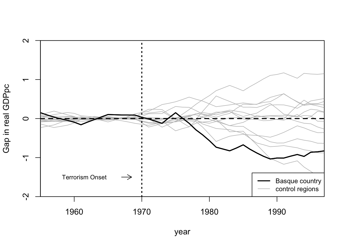

Concluding remarks

Synthetic control methods can be used to estimate causal effects.
These methods also enable precise inferential techniques when used with the Synth package in R.
Several enhancements to Synth are currently under development.
A regression-based method is being tested to populate the entire \(V\) matrix, not just its diagonal.
A version of Synth is being refined to select the \(W\) weights that best fit multiple outcome variables at the same time.
Work is in progress on a version of Synth that can handle multiple treatments introduced over a period of time.

References

Abadie, A., Diamond, A., & Hainmueller, J. (2011). Synth: An R Package for Synthetic Control Methods in Comparative Case Studies. Journal of Statistical Software, 42(13), 1–17. https://doi.org/10.18637/jss.v042.i13

Abadie A, Diamond A, Hainmueller J (2010). “Synthetic Control Methods for Comparative Case Studies: Estimating the Effect of California’s Tobacco Control Program.” Journal of the American Statistical Association, 105(490), 493-505.

Abadie A, Gardeazabal J (2003). “The Economic Costs of Conflict: A Case Study of the Basque Country.” American Economic Review, 93(1), 112-132.

Bertrand M, Duflo E, Mullainathan S (2004). “How Much Should We Trust Differences-inDifferences Estimates?” Quarterly Journal of Economics, 119(1), 249-275.

Karatzoglou A, Smola A, Hornik K, Zeileis A (2004). “kernlab - An S4 Package for Kernel Methods in R.” Journal of Statistical Software, 11(9), 1-20. URL http://www . jstatsoft. org/v11/i09/.

Lehmann EL (1997). Testing Statistical Hypotheses. 2nd edition. University of California Press, Berkeley.

Mebane, Jr WR, Sekhon JS (2011). “Genetic Optimization Using Derivatives: The rgenoud Package for R.” Journal of Statistical Software, 42(11), 1-26. URL http : //www . jstatsoft . org/v42/i11/.

Introduction

Synthetic control methods

Implementation of the Synth package

Using dataprep()

Running synth()